pm-remez documentation#

pm-remez is a modern Rust implementation of the Parks-McClellan Remez exchange algorithm. It can be used as a Rust library and as a Python package via its Python bindings.

pm-remez supports the design of FIR filters with even symmetry and odd symmetry, and with an even number of taps and an odd number of taps, by reducing all these cases to the even symmetry odd number of taps case. The desired frequency response in each band, as well as the weights, can be defined as arbitrary functions. The Python package can use double-precision IEEE 754 floating-point numbers for calculations, as well as the higher precision num-bigfloat library. This can be used to solve numerically challenging problems that are difficult to solve using double-precision arithmetic.

The implementation draws ideas from a paper by S.I. Filip to make the algorithm robust against numerical errors. These ideas include the use of Chebyshev proxy root finding to find the extrema of the weighted error function in the Remez exchange step.

pm_remez.remez(numtaps, bands, desired, *, weight=None, symmetry='even', maxiter=100, fs=1.0, bigfloat=False)#

Calculate the minimax optimal filter using the Parks-McClellan Remez exchange algorithm.

Calculate the filter-coefficients for the even-symmetric or odd-symmetric finite impulse response (FIR) filter whose transfer function minimizes the maximum weighted error between the desired gain and the realized gain in the specified frequency bands using the Parks-McClellan algorithm.

The API of this function is heavily inspired by scipy.signal.remez() to remain compatible with basic usage of SciPy’s remez implementation.

Unlike SciPy’s Remez algorithm, this function supports indicating non-constant desired gain and weight in each of the bands. The gain or weight can be indicated in three possible ways:

As a scalar. This indicates a constant value in all the band.
As an array_like containing two elements. This indicates a linear slope in the band. The first element of the array_like indicates the value at the beginning of the band, and the second element of the array_like indicates the value at the end of the band.
As a callable. This indicates an arbitrary function that will be evaluated by the algorithm as required. The function must be continuous in all the points of the band.

Parameters:

numtapsint: The desired number of taps in the filter.
bandsarray_like: A sequence defining the band edges. The length of the sequence must be even. Every pair of elements in the sequence indicate the edges of one of the bands. All elements must be non-negative and less than half the sampling frequency as given by fs.
desiredarray_like: A sequence half the size of bands containing the desired gain in each of the specified bands. The elements in the sequence represent either a constant, a linear slope, or an arbitrary function as described above.
weightarray_like, optional: A sequence half the size of bands indicating the weight function in each band. The elements in the sequence represent either a constant, a linear slope, or an arbitrary function as described above. By default, a constant weight of 1 is given to all the bands.
symmetry{‘even’, ‘odd’}, optional: The symmetry of the filter. The default is even.
maxiterint, optional: Maximum number of iterations of the algorithm. Default is 100.
fsfloat, optional: The sampling frequency of the signal. Default is 1.0.
bigfloatbool, optional: Use num_bigfloat for all the internal calculations. This is much slower than using float64, but it allows some ill-conditioned problems to converge. Default is False.

Returns:

impulse_responseList[float]: A list containing the coefficients of the optimal FIR filter.
weighted_errorfloat: The maximum absolute value of the weighted error achieved by the optimal filter.
extremal_freqsList[float]: A list containing the extremal frequencies of the optimal filter. These are frequencies at which the maximum weighted error is reached (or almost) reached. The frequencies are used as nodes for polynomial interpolation.
num_iterationsint: The number of iterations that the Parks-McClellan algorithm required to converge to the optimal filter.
flatnessfloat: A metric used to assess if the algorithm has converged. It is defined as the difference between the maximum absolute value of the weighted error over all the extremal frequencies minus the minimum absolute value of the weighted error over all the extremal frequencies, divided by the maximum absolute value of the weighted error over all the extremal frequencies.

Examples

The following examples both illustrate the capabilities of pm-remez and also serve as a guide that shows how to design commonly used types of FIR filters. All the examples use scipy.signal.freqz() to compute the frequency response of the FIR filter, which is then plotted. These imports are required.

>>> import pm_remez
>>> import numpy as np
>>> import scipy
>>> import matplotlib.pyplot as plt

Lowpass filters

A common type of lowpass filter is an anti-alias filter used for decimation. Assuming fs = 1, the cut-off frequency of such filter is at 0.5 / decimation, where decimation is the decimation factor. The same filter can also be used as an anti-alias filter for interpolation. A way to define the passband and stopband of the filter is with a transition_bandwidth parameter, which indicates what fraction of the output Nyquist frequency range is not part of the filter passband, and thus not usable due to filter roll-off and aliasing. Here is a generic function to design this type of filter.

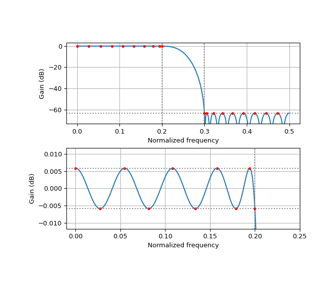
>>> def design_antialias_lowpass(decimation, transition_bandwidth, numtaps,
>>>                              stopband_weight=1.0, one_over_f=False,
>>>                              bigfloat=False, worN=4096):
>>>     passband_end = 0.5 * (1 - transition_bandwidth) / decimation
>>>     stopband_start = 0.5 * (1 + transition_bandwidth) / decimation
>>>     # Stopband weight is a constant or linear slope depending
>>>     # on one_over_f parameter.
>>>     sweight = ((stopband_weight, stopband_weight * 0.5 / stopband_start)
>>>                if one_over_f else stopband_weight)
>>>     design = pm_remez.remez(
>>>                  numtaps, [0, passband_end, stopband_start, 0.5],
>>>                  [1, 0], weight=[1, sweight], bigfloat=bigfloat)
>>>
>>>     # Compute and plot the frequency response of the filter
>>>     w, h = scipy.signal.freqz(design.impulse_response, [1], worN=worN, fs=1)
>>>     fig, axs = plt.subplots(2, 1, figsize=(7, 6))
>>>     for j, ax in enumerate(axs):
>>>         ax.plot(w, 20 * np.log10(np.abs(h)))
>>>         att_db = 20 * np.log10(design.weighted_error / stopband_weight)
>>>         ripple_db = 20 * np.log10(1 + design.weighted_error)
>>>         for sign in [-1, 1]:
>>>             ax.axvline(x=0.5 * (1 + sign * transition_bandwidth) / decimation,
>>>                        color='grey', linestyle=':')
>>>         ax.axhline(y=att_db, color='grey', linestyle=':')
>>>         for f in design.extremal_freqs:
>>>             hf = 20 * np.log10(np.abs(np.sum(
>>>                      np.array(design.impulse_response)
>>>                      * np.exp(1j * 2 * np.pi * f
>>>                      * np.arange(len(design.impulse_response))))))
>>>             ax.plot(f, hf, '.', color='red')
>>>         if j == 0:
>>>             max_att = att_db
>>>             if one_over_f:
>>>                 max_att -= 20 * np.log10(0.5 / stopband_start)
>>>             ax.set_ylim((max_att - 10, 3))
>>>         else:
>>>             ax.set_ylim((-2 * ripple_db, 2 * ripple_db))
>>>             ax.set_xlim((-0.02 / decimation, 0.5 / decimation))
>>>             ax.axhline(y=ripple_db, color='grey', linestyle=':')
>>>             ax.axhline(y=20 * np.log10(1 - design.weighted_error),
>>>                        color='grey', linestyle=':')
>>>         ax.grid()
>>>         ax.set_xlabel('Normalized frequency')
>>>         ax.set_ylabel('Gain (dB)')
>>>     plt.subplots_adjust(hspace=0.3)
>>>
>>>     return design

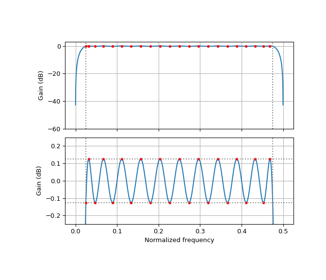
A simple design for a 20% transition bandwidth with 35 taps achieves a stopband attenuation better than -60 dB. The extremal frequencies of the optimal filter are marked with red dots.

>>> design_antialias_lowpass(2, 0.2, 35)
>>> plt.show()

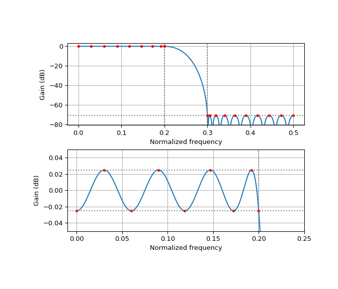
The stopband attenuation can be improved at the cost of passband ripple by increasing the relative weight applied to the stopband.

>>> design_antialias_lowpass(2, 0.2, 35, stopband_weight=10)
>>> plt.show()

Some authors recommend making the amplitude response decay as 1/f in the stopband. This helps to reduce the integrated stopband levels for high decimation factor filters, and makes it easier for the filter to still satisfy the stopband attenuation requirements after the coefficients have been quantized to fixed point. The way to design this kind of filter is by using a linear slope function as the stopband weight. This is enabled by setting one_over_f=True in this example function. Here we design a decimate by 4 filter to illustrate the 1/f decay bettery.

>>> design_antialias_lowpass(4, 0.2, 67, stopband_weight=10, one_over_f=True)
>>> plt.show()

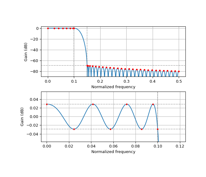
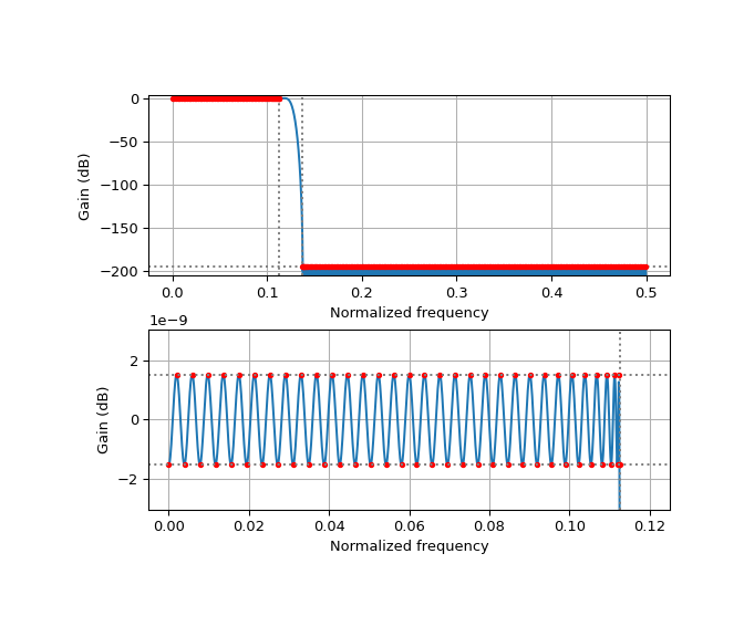
A filter with a large number of taps is able to achieve a narrow transition bandwidth with good stopband attenuation, and this is usually the reason why a larger number of taps might be required in a filter. However, if a filter with many taps is designed for a resonably large transition bandwidth, it is able to achieve a very large stopband attenuation and passband flatness. This makes the numerical problem ill-conditioned. pm-remez can use the num_bigfloat library to solve this kinds of problems. For example, here is a 512 tap filter with a transition bandwidth of 10% that achieves almost -200 dB stopband attenuation. This kind of filter is rarely useful in practice.

>>> design_antialias_lowpass(4, 0.1, 512, bigfloat=True)
>>> plt.show()

Polyphase filterbank prototype filters

A particular kind of anti-alias lowpass filter is the prototype filter for a polyphase filterbank (polyphase channelizer). These are filters for a decimation factor equal to the number of channels, which is usually a relatively large power of two when the polyphase filterbank is used for spectral analysis. The number of taps is equal to an integer (usually small) times the number of channels.

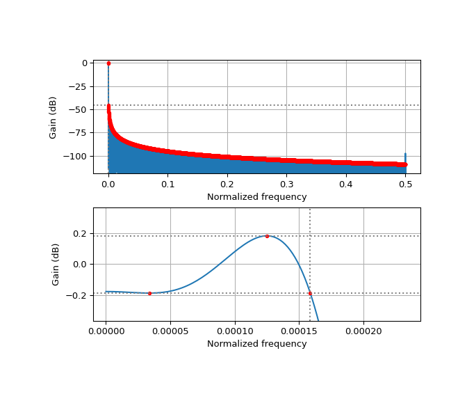
The following example designs a prototype filter for a 2048 channel polyphase filterbank with 6 taps per channel and a transition bandwidth of 35%. A custom stopband weight and 1/f decay are used for best results. This filter is close to the limits of what can be design with pm-remez without running into numerical problems (even with bigfloat=True). Increasing the number of channels to 4096, or increasing the stopband weight, will make the algorithm fail.

A prototype filter for a certain number of channels can be turned into a prototype filter for a larger number of channels with the same number of taps per channel by interpolation of the prototype filter taps. The resulting filter will not be optimal in the minimax sense, but it will be close if the initial filter was designed for a large number of taps. This is a practical way to design prototype filters for more than 2048 channels.

>>> num_channels = 2048
>>> taps_per_channel = 6
>>> design = design_antialias_lowpass(num_channels, 0.35, num_channels * taps_per_channel,
>>>                                   stopband_weight=4, one_over_f=True, worN=2**18)
>>> plt.show()

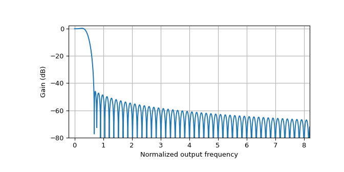
Here is a plot that shows the shape of the passband more clearly. The points where the normalized output frequency is an integer correspond to the centers of the filterbank channels.

>>> w, h = scipy.signal.freqz(design.impulse_response, [1], worN=2**18, fs=1)
>>> plt.plot(w * num_channels, 20*np.log10(np.abs(h)))
>>> plt.xlim((-0.2, 8 + 0.2))
>>> plt.ylim((-80, 2))
>>> plt.grid()
>>> plt.xlabel('Normalized output frequency')
>>> plt.ylabel('Gain (dB)')
>>> plt.show()

Bandpass filters

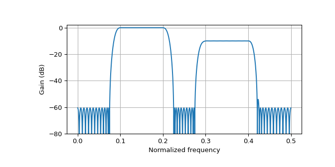
Bandpass filters are less common than lowpass filter, but they can also be easily designed with the Parks-McClellan algorithm. The following example designs a filter with two passbands, one with 0 dB of gain and another passband with -10 dB of gain. While the amplitude response of an optimal lowpass filter in the transition band is always decreasing, bandpass filter and other types of filters can have more complicated and sometimes undesirable behavior in the transition bands, because the minimax optimization problem does not constrain the response in the transition bands.

>>> design = pm_remez.remez(135, [0, 0.075, 0.1, 0.2, 0.225, 0.275, 0.3, 0.4, 0.425, 0.5],
>>>                         [0, 1, 0, np.sqrt(1/10), 0])
>>> w, h = scipy.signal.freqz(design.impulse_response, [1], worN=4096, fs=1)
>>> plt.plot(w, 20*np.log10(np.abs(h)))
>>> plt.ylim((-80, 2))
>>> plt.grid()
>>> plt.xlabel('Normalized frequency')
>>> plt.ylabel('Gain (dB)')
>>> plt.show()

CIC compensation filters

CIC filters are rather popular for decimation and interpolation because they do not require multipliers. The frequency response of an M-stage CIC filter used for decimation by a factor of D is (normalized to unit gain)

\[\left|\frac{\sin(\pi f D)}{D \sin(\pi f)}\right|^M.\]

On its own, a CIC filter is not so good as an anti-alias filter. The passband is far from flat, and the stopband attenuation is not high enough. For this reason, a CIC is usually followed by a FIR decimator with a small decimation factor such as 2, 3, or 4. The FIR decimator limits the part of the passband that is used to the flatter central region and attenuates the regions of the spectrum where the CIC stopband is worst.

Sometimes, this FIR decimator is designed as a CIC compensation filter, by having a passband response that is equal to the inverse of the CIC filter response. In this way, the passband of the combined filter is flattened.

Compensation filters can be designed with pm-remez by using a Python function or lambda to define the desired passband response. The following example is a general function to design and plot CIC compensation filters.

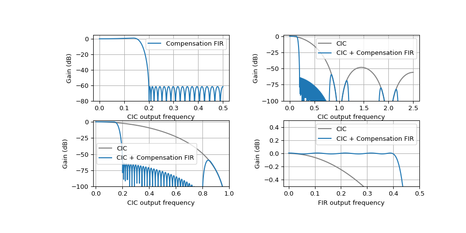
>>> def design_cic_compensation(cic_stages, cic_decimation,
>>>                             decimation, transition_bandwidth, numtaps,
>>>                             cic_decimation_independent=False,
>>>                             cic_decimation_for_compensation=None):
>>>     passband_end = 0.5 * (1 - transition_bandwidth) / decimation
>>>     stopband_start = 0.5 * (1 + transition_bandwidth) / decimation
>>>
>>>     def desired(f):
>>>         if f < 1e-3:
>>>             # avoid math errors near f = 0
>>>             return 1
>>>         if cic_decimation_independent:
>>>             one_stage = np.pi * f / np.sin(np.pi * f)
>>>         else:
>>>             dec = (cic_decimation_for_compensation
>>>                    if cic_decimation_for_compensation is not None
>>>                    else cic_decimation)
>>>             one_stage = dec * np.sin(np.pi * f / dec) / np.sin(np.pi * f)
>>>         return one_stage**cic_stages
>>>
>>>     design = pm_remez.remez(numtaps, [0, passband_end, stopband_start, 0.5],
>>>                             [desired, 0])
>>>
>>>     # Plot response of the FIR filter
>>>     fig, axs = plt.subplots(2, 2, figsize=(10, 5))
>>>     axs = axs.ravel()
>>>     w, h = scipy.signal.freqz(design.impulse_response, [1], worN=4096, fs=1)
>>>     axs[0].plot(w, 20*np.log10(np.abs(h)), label='Compensation FIR')
>>>     axs[0].set_ylim((-80, 5))
>>>
>>>     # Compute taps of the CIC filter (understood as a FIR filter)
>>>     cic_taps = np.ones(1)
>>>     for _ in range(cic_stages):
>>>         cic_taps = np.convolve(cic_taps, np.ones(cic_decimation))
>>>     cic_taps /= np.sum(cic_taps)
>>>
>>>     # Compute taps of the combination of CIC filter + Compenstation FIR
>>>     fir_taps_zero_packed = np.zeros((numtaps, cic_decimation))
>>>     fir_taps_zero_packed[:, 0] = design.impulse_response
>>>     fir_taps_zero_packed = fir_taps_zero_packed.ravel()
>>>     total_taps = np.convolve(cic_taps, fir_taps_zero_packed)
>>>
>>>     # Plot response of CIC and combined filter
>>>     w, h_cic = scipy.signal.freqz(cic_taps, [1], worN=4096, fs=1)
>>>     w, h_total = scipy.signal.freqz(total_taps, [1], worN=4096, fs=1)
>>>     for j in range(1, 4):
>>>         xaxis = (w * cic_decimation * decimation
>>>                  if j == 3 else w * cic_decimation)
>>>         axs[j].plot(xaxis, 20*np.log10(np.abs(h_cic)), 'grey', label='CIC')
>>>         axs[j].plot(xaxis, 20*np.log10(np.abs(h_total)), label='CIC + Compensation FIR')
>>>         axs[j].set_ylim((-100, 2))
>>>
>>>     axs[2].set_xlim((-0.02, 1))
>>>     axs[3].set_xlim((-0.02, 0.5))
>>>     axs[3].set_ylim((-0.5, 0.5))
>>>
>>>     for j, ax in enumerate(axs):
>>>         ax.grid()
>>>         ax.set_xlabel('FIR output frequency' if j == len(axs) - 1
>>>                       else 'CIC output frequency')
>>>         ax.set_ylabel('Gain (dB)')
>>>         ax.legend()
>>>
>>>     plt.subplots_adjust(hspace=0.3)
>>>
>>>     return design

This designs a compensation filter for a 4-stage CIC that decimates by 5. The compensation FIR decimates by 3 and has a transition bandwidth of 20%.

>>> design_cic_compensation(4, 5, 3, 0.2, 53)
>>> plt.show()

Another attractive characteristic of CIC filters is that the same CIC filter can be used for different decimation factors just by changing the rate at which output samples are strobed. However, the frequency response of the CIC filter depends on the decimation factor D, so the compensation filter also depends on D. Putting \(s = f D\), which represents the normalized frequency at the input of the compensation FIR, when D is large, the CIC response can be approximated as

\[\left|\frac{\sin(\pi f D)}{\sin(\pi f)}\right|^M = \left|\frac{\sin(\pi s)}{D \sin(\pi s / D)}\right|^M \approx \left|\frac{\sin(\pi s)}{\pi s}\right|^M,\]

which is independent of D.

The design_cic_compensation example has a parameter cic_decimation_independent that can be used to design a compensation FIR that is independent of the CIC decimation by using this approximation. When the CIC is configured for a small decimation factor, the decimation-independent compensation will not match completely the CIC response, and the resulting passband will be slightly not flat.

>>> design_cic_compensation(4, 5, 3, 0.2, 53, cic_decimation_independent=True)
>>> plt.show()

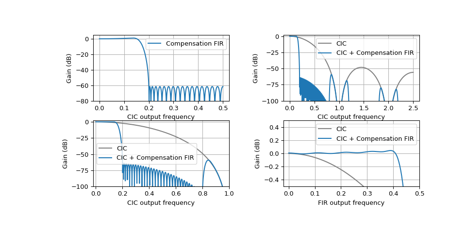
If a CIC filter is primarily to be used for small decimation factors, another possible approach to obtain a compensation FIR to be used for all the decimation factors is simply to fix the value of D that is used to design the FIR to one of the small CIC decimation factors that are used more frequently.

The design_cic_compensation function has a parameter cic_decimation_for_compensation that can be used to force the compensation FIR to be designed for the given value of D. This is used to evaluate the performance of the combined filter when the CIC is set to a different decimation factor. For instance, the following designs a compensation FIR for D = 3 and evaluates it with the CIC set to a decimation factor of 5.

>>> design_cic_compensation(4, 5, 3, 0.2, 53, cic_decimation_for_compensation=3)
>>> plt.show()

Hilbert filters

Different sources in the signal processing literature use the term Hilbert filter to refer to different, but related, types of FIR filters. Some sources (including most sources which speak of Hilbert filters in the context of the Parks-McClellan algorithm) call Hilbert filter to a FIR filter that tries to approximate the Hilbert transform. The frequency response of such an ideal Hilbert filter is \(-i\) for \(f > 0\) and \(i\) for \(f < 0\). Therefore, the filter shifts the phase of a signal backwards or forwards by 90 degrees according to whether the frequency of the signal is positive or negative respectively.

Such an ideal Hilbert filter cannot be realized as a FIR filter, because the frequency response is not continous among other reasons. FIR filters with real coefficients, odd symmetry, and an odd number of taps have a frequency response which is a purely imaginary odd function. Therefore, an all-pass FIR filter with those properties that has an amplitude response close to one for all frequencies except near zero and the Nyquist frequency is a good approximation of a Hilbert filter (the sign of all the FIR taps might need to be flipped to make the imaginary part of the frequency response positive for negative frequencies).

Other sources in the literature use the term Hilbert filter to refer to what in mathematics is called the Riesz projection. The Riesz projection is an ideal filter whose frequency response is one for \(f > 0\) and zero for \(f < 0\). Such a filter acts as an all-pass filter for signals of positive frequencies and removes all the signals of negative frequencies. This filter is often used in the context of transforming a real signal into a complex signal, since the filter removes the negative frequency (mirrored) part of the spectrum of the real signal. An example of this application is the GNU Radio Hilbert block.

The Hilbert transform and the Riesz projection are closely related. If we denote by \(H\) the Hilbert transform and by \(P\) the Riesz projection, we see that \(P = (I + iH) / 2\), where \(I\) denotes the identity transformation. A FIR filter with complex-valued taps that approximates the Riesz projection can be built from such a Hilbert FIR filter by setting the imaginary part of the taps to one half of the values of the Hilbert FIR filter taps, and the real part of the taps to zero except in the central tap, where it is set to the value 0.5.

In some implementations of the Parks-McClellan algorithm, including in scipy.signal.remez(), Hilbert filters are treated as a special type of filter. In pm-remez, Hilbert filters are not a special case. They are designed as filters with an odd number of taps, and with odd symmetry, by using the parameter symmetry = 'odd'. Since such a FIR filter must have a frequency response of zero at DC and at the Nyquist frequency, the desired response needs to be set to zero at these frequencies. The filter is designed as an all-pass filter that has a band covering almost from DC to the Nyquist frequency and desired gain of one.

Here is an example function that designs and plots Hilbert filters. The transition_bandwidth parameter corresponds to the fraction of the bandwidth that is used to leave a gap between the all-pass band and DC and the Nyquist frequency.

>>> def design_hilbert(transition_bandwidth, numtaps):
>>>     assert numtaps % 2 == 1, "numtaps must be odd"
>>>     allpass_begin = 0.25 * transition_bandwidth
>>>     allpass_end = 0.5 - 0.25 * transition_bandwidth
>>>     design = pm_remez.remez(numtaps, [allpass_begin, allpass_end], [1], symmetry='odd')
>>>
>>>     # Compute and plot the frequency response of the filter
>>>     w, h = scipy.signal.freqz(design.impulse_response, [1], worN=4096, fs=1)
>>>     fig, axs = plt.subplots(2, 1, figsize=(7, 6), sharex=True)
>>>     for j, ax in enumerate(axs):
>>>         ax.plot(w, 20 * np.log10(np.abs(h)))
>>>         ripple_db = 20 * np.log10(1 + design.weighted_error)
>>>         for x in [allpass_begin, allpass_end]:
>>>             ax.axvline(x=x, color='grey', linestyle=':')
>>>         for f in design.extremal_freqs:
>>>             hf = 20 * np.log10(np.abs(np.sum(
>>>                      np.array(design.impulse_response)
>>>                      * np.exp(1j * 2 * np.pi * f
>>>                      * np.arange(len(design.impulse_response))))))
>>>             ax.plot(f, hf, '.', color='red')
>>>         if j == 0:
>>>             ax.set_ylim((-60, 3))
>>>         else:
>>>             ax.set_ylim((-2 * ripple_db, 2 * ripple_db))
>>>             ax.axhline(y=ripple_db, color='grey', linestyle=':')
>>>             ax.axhline(y=20 * np.log10(1 - design.weighted_error),
>>>                        color='grey', linestyle=':')
>>>         ax.grid()
>>>         ax.set_ylabel('Gain (dB)')
>>>     axs[-1].set_xlabel('Normalized frequency')
>>>     plt.subplots_adjust(hspace=0.1)
>>>
>>>     return design

This designs a Hilbert filter with a transition bandwidth of 10%. The passband flatness can be improved by increasing the number of taps.

>>> design_hilbert(0.1, 43)
>>> plt.show()

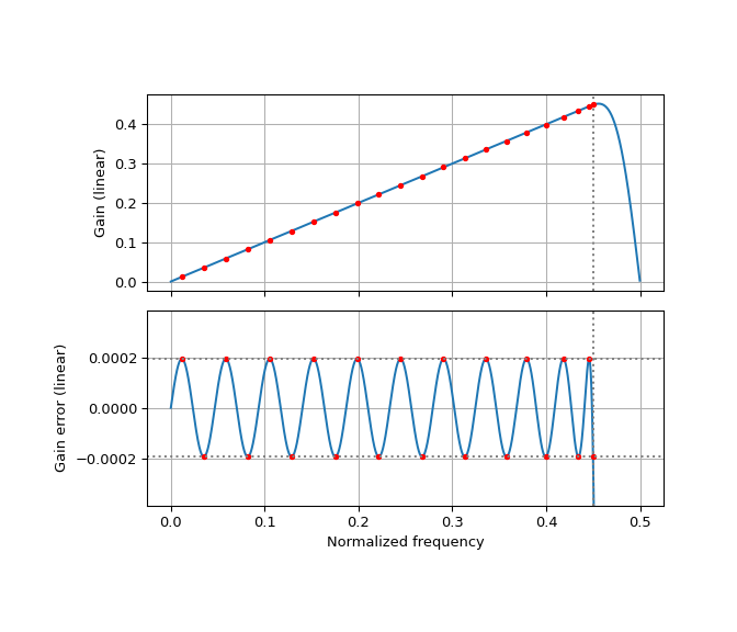
Differentiator filters

The ideal frequency or response of a differentiator filter at frequency \(f\) is \(if\) (or a multiple of this). A differentiator FIR filter can be designed as a filter with odd symmetry and an odd number of taps (since the frequency response of such a filter is a purely imaginary odd function) and with a desired response that has a linear slope proportional to \(f\). Since this kind of FIR filter must have a frequency response of zero a the Nyquist frequency (and also at DC), it is necessary to leave a gap between the band where the desired response is set and the Nyquist frequency.

As for Hilbert filters, in some implementations of the Parks-McClellan algorithm, including in scipy.signal.remez(), differentiator filters are treated as a special type of filter, but in pm-remez they are not a special case. A differentiator filter can be designed with pm-remez by setting a linear slope as desired response in the passband.

The following example designs and plots a differentiator filter. The transition_bandwidth parameter determines the fraction of the bandwidth that is used as a gap between the band where the desired response is enforced and the Nyquist frequency.

>>> def design_differentiator(transition_bandwidth, numtaps):
>>>     assert numtaps % 2 == 1, "numtaps must be odd"
>>>     allpass_end = 0.5 - 0.5 * transition_bandwidth
>>>     design = pm_remez.remez(numtaps, [0, allpass_end], [(0, allpass_end)], symmetry='odd')
>>>
>>>     # Compute and plot the frequency response of the filter
>>>     w, h = scipy.signal.freqz(design.impulse_response, [1], worN=4096, fs=1)
>>>     fig, axs = plt.subplots(2, 1, figsize=(7, 6), sharex=True)
>>>     axs[0].plot(w, np.abs(h))
>>>     axs[1].plot(w, np.abs(h) - w)
>>>     ripple = design.weighted_error
>>>     axs[1].set_ylim((-2 * ripple, 2 * ripple))
>>>     for j, ax in enumerate(axs):
>>>         ax.axvline(x=allpass_end, color='grey', linestyle=':')
>>>         for f in design.extremal_freqs:
>>>             hf = np.abs(np.sum(np.array(design.impulse_response)
>>>                                * np.exp(1j * 2 * np.pi * f
>>>                                * np.arange(len(design.impulse_response)))))
>>>             if j == 1:
>>>                 hf = hf - f
>>>             ax.plot(f, hf, '.', color='red')
>>>         ax.grid()
>>>     axs[0].set_ylabel('Gain (linear)')
>>>     axs[1].set_ylabel('Gain error (linear)')
>>>     for sign in [-1, 1]:
>>>         axs[1].axhline(y=sign*ripple, color='grey', linestyle=':')
>>>     axs[-1].set_xlabel('Normalized frequency')
>>>     plt.subplots_adjust(hspace=0.1)
>>>     return design

Here is a differentiator filter with a transition banwdith of 10%. The gain error ripple can be decreased by increasing the number of taps.

>>> des = design_differentiator(0.1, 43)
>>> plt.show()